Sunday, November 8, 2015

Blog Post 28, WS 9.1, Problem 1: Deriving Friedmann

The Friedmann equations describe the dynamics of a universe filled with mass. We will derive them Newtonian Mechanics. Consider a universe filled with matter which has a mass density \(rho(t)\). Note that as the universe expands or contracts, the density of the matter changes with time, which is why it is a function of time t.
Now consider a mass shell of radius R within this universe. The total mass of the matter enclosed by this shell is M. In the case we consider (homogeneous and isotropic universe), there is no shell crossing, so M is a constant.

WARNING: MATH AHEAD

(a) Find the shell's acceleration.
This is pretty simple.  We will use Newton's gravity equation.
\[F_g=\frac{GMm}{R^2}\]
We know that \(\dot(v)=F/m\), so: 
\[\dot{v}=\frac{GM}{R^2}\]

(b) Convert to energy.
We will use the quick trick of multiplying both sides by velocity and integrating.
\[\dot{v}v=\frac{GMv}{R^2}\]
\[vdv=\frac{GMdR}{R^2}\]
\[\frac{1}{2}v^2=\frac{GM}{R}+C\]
\[\frac{1}{2}\dot{R}^2-\frac{GM}{R}=C\]

(c) Express using mass density.
\[M=\frac{4}{3}\pi R^3 \rho\]
\[\frac{1}{2}\dot{R}^2-\frac{G(\frac{4}{3}\pi R^3 \rho)}{R}=C\]
\[\frac{1}{2}\dot{R}^2-\frac{G4\pi R^2 \rho}{3}=C\]
\[\left(\frac{\dot{R}}{R}\right)^2=\frac{8\pi G \rho}{3}+\frac{2C}{R^2}\]

(d,e) Express using R=a(t)r where r is the coming radius of the sphere.
\[\left(\frac{\dot{R}}{R}\right)^2=\frac{8\pi G \rho}{3}+\frac{2C}{R^2}\]
\[\left(\frac{\dot{a}}{a}\right)^2=\frac{8\pi G \rho}{3}+\frac{2C}{a^2 r^2}\]

(f) In the last worksheet we showed that \(H(t) = \frac{\dot{a}}{a}\).  Express the First Friedmann Equation using this term.  We can also turn \(2c/r^2\) into \(-kc^2\), a curvature term.
\[\left(\frac{\dot{a}}{a}\right)^2=\frac{8\pi G \rho}{3}+\frac{2C}{a^2 r^2}\]
\[\boxed{H^2=\frac{kc^2}{a^2}+\frac{8\pi G \rho}{3}}\]

(g)  Derive the Second Friedmann Equation by expressing the acceleration of our initial shell in terms of the universal density.
From before we established:
\[\dot{v}=\frac{GM}{R^2}\]
\[\ddot{R}=\frac{4}{3}GM\pi R \rho\]
\[\boxed{\frac{\ddot{a}}{a}=-\frac{4}{3}\pi G \rho}\]

These Friedmann equations only apply to a universe that contains only matter without any pressure.  The more extensive Friedmann equations come from General Relativity.  

I worked with B. Brzycki, G. Grell, and N. James on this problem.

Sunday, November 1, 2015

Blog Post 27, WS 8.1, Problem 3: Hubble Flow and Constant


It is not strictly correct to associate this ubiquitous distance-dependent redshift we observe with the velocity of the galaxies (at very large separations, Hubble’s Law gives ‘velocities’ that exceeds the speed of light and becomes poorly defined). What we have measured is the cosmological redshift, which is actually due to the overall expansion of the universe itself. This phenomenon is dubbed the Hubble Flow, and it is due to space itself being stretched in an expanding universe.

Since everything seems to be getting away from us, you might be tempted to imagine we are located at the centre of this expansion. But, as you explored in the opening thought experiment, in actuality, everything is rushing away from everything else, everywhere in the universe, in the same way. So, an alien astronomer observing the motion of galaxies in its locality would arrive at the same conclusions we do.

In cosmology, the scale factor, a(t), is a dimensionless parameter that characterizes the size of the universe and the amount of space in between grid points in the universe at time t. In the current epoch, t = t0 and a(t0) = 1. a(t) is a function of time. It changes over time, and it was smaller in the past (since the universe is expanding). This means that two galaxies in the Hubble Flow separated by distance d0 = d(t0) in the present were d(t)= a(t)d0 apart at time t.

The Hubble Constant is also a function of time, and is defined so as to characterize the fractional rate of change of the scale factor:
\[H(t)=\frac{1}{a(t)} \frac{da}{dt}\rvert_t\]
and the Hubble Law is locally valid for any t:
\[v=H(t)d\]
where v is the relative recessional velocity between two points and d the distance that separates them.

(a) Assume the rate of expansion, \(\dot{a}= da/dt\), has been constant for all time. How long ago was the Big Bang (i.e. when a(t=0)=0)? How does this compare with the age of the oldest globular clusters (~12 Gyr)? What you will calculate is known as the Hubble Time.

(b) What is the size of the observable universe? What you will calculate is known as the Hubble Length.

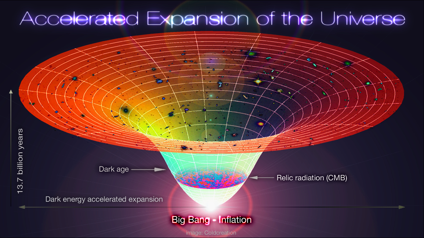
https://upload.wikimedia.org/wikipedia/commons/c/c2/Lambda-Cold_Dark_Matter,_Accelerated_Expansion_of_the_Universe,_Big_Bang-Inflation.jpg

(a) Assume the rate of expansion, \(\dot{a}= da/dt\), has been constant for all time. How long ago was the Big Bang (i.e. when a(t=0)=0)? How does this compare with the age of the oldest globular clusters (~12 Gyr)? What you will calculate is known as the Hubble Time. 

It's time for some math.
We want to solve for \(t_0\).
Let's start with the given equation:
\[H(t)=\frac{1}{a(t)} \frac{da}{dt}\]
We can define \(da/dt=\dot{a}\).
\[H(t)=\frac{1}{a(t)} \dot{a}\]
\[H_0=\frac{\dot{a}}{a(t_0)}\]
We are also told that \(a(t_0)=1\), thus:
\[H_0=\frac{\dot{a}}{1}\]
\[H_0=\dot{a}\]
We will now change \(\dot{a}\) back to \(da/dt\).
\[H_0=\frac{da}{dt}\]
Let's integrate.
\[H_0 dt=da\]
\[\int^{t_0}_0 H_0 dt=\int^{a(t_0)=1}_0 da\]
\[H_0 t_0=1\]
\[t_0=H_0^{-1}\]
We found in a previous problem that \(H_0=68 km/s/Mpc\), thus:
\[\boxed{t_H=4.6\times 10^{17} sec=14.4 billion years}\]
This is the Hubble time.

(b) What is the size of the observable universe? What you will calculate is known as the Hubble Length. 

The fastest traveling entity in the universe is light, thus the Hubble distance can be expressed as:
\[D_H=t_H c\]
\[D_H=(4.6\times 10^{17} sec)\times (3\times 10^10 cm\sec)\]
\[\boxed{D_H=1.36\times 10^{28}cm=4400Mpc=4.4Gpc}\]

Lengths of this scale are certainly, astronomical.  
(Pro-tip: click the link).

I worked on this problem with B. Brzycki, G. Grell, N. James.

Blog Post 26, WS 8.1, Problem 1: Spatial Expansion

Before we dive into the Hubble Flow, let’s do a thought experiment. Pretend that there is an infinitely long series of balls sitting in a row. Imagine that during a time interval ∆t the space between each ball increases by ∆x. 

(a) Look at the shaded ball, Ball C, in the figure above. Imagine that Ball C is sitting still (so we are in the reference frame of Ball C). What is the distance to Ball D after time ∆t? What about Ball B?

(b) What are the distances from Ball C to Ball A and Ball E?

(c) Write a general expression for the distance to a ball N balls away from Ball C after time ∆t. Interpret your finding.

(d) Write the velocity of a ball N balls away from Ball C during ∆t. Interpret your finding.

This problem is very hypothetical but its a great introduction into spatial expansion of the universe.

(a) Look at the shaded ball, Ball C, in the figure above. Imagine that Ball C is sitting still (so we are in the reference frame of Ball C). What is the distance to Ball D after time ∆t? What about Ball B? 

This pretty easy, the problem says that the distance increases by \(\Delta\)x every \(\Delta\)t, also D and B are both 1 ball away from C. Thus:
\[d_{D,C}(\Delta t)=d_{B,C}(\Delta t)=\Delta x\]

(b) What are the distances from Ball C to Ball A and Ball E?

This requires a little bit more thought.  Since A and E are two balls away, each will move a distance 2\(\Delta\)x.  Thus:
\[d_{E,C}(\Delta t)=d_{A,C}(\Delta t)=2\Delta x\]

(c) Write a general expression for the distance to a ball N balls away from Ball C after time ∆t. Interpret your finding. 
Let's look at our last two answers.  The distance travelled by a ball seems to be proportionate to the number of balls between the two endpoints.  Thus, we can write:
\[d_N(\Delta t)=N\Delta x\]
This implies that the further away an object is, the more it moves away in a time-step.

(d) Write the velocity of a ball N balls away from Ball C during ∆t. Interpret your finding. 
Velocity can be written as \(\frac{\Delta x}{\Delta t}\).  Thus we can modify our previous expression:
\[v_N(\Delta t)=N\frac{\Delta x}{\Delta t}=N\Delta v\]
Let's interpret our findings.  We can come up with 2 general rules for our forceless expanding space:
1. Objects always move away for each other
2. The farther away an object is, he faster it moves further away.  

These rules hold true in our real universe provided that no other forces act upon the objects.  For instance, distant galaxies and quasars are moving away from us faster and faster every day.  However, 
nearby galaxies such as Andromeda are close enough to be affected by the force of gravity, thus Andromeda is ready to collide with us in the Milkomeda collision.  This spatial expansion is even occurring on the space between our cells and between our very atoms, but the fundamental forces are more than strong enough to make spatial expansion not even register of such small scales.

I worked with B. Brzycki, G. Grell, and N. James on this problem.
Blog Post 25, WS 7.2, Problem 5: More Quasar Redshift


You may also have noticed some weak “dips” (or absorption features) in the spectrum: 

a) Suggest some plausible origins for these features. By way of inspiration, you may want to consider what might occur if the bright light from this quasar’s accretion disk encounters some gaseous material on its way to Earth. That gaseous material will definitely contain hydrogen, and those hydrogen atoms will probably have electrons occupying the lowest allowed energy state. 

(b) A spectrum of a different quasar is shown below. Assuming the strongest emission line you see here is due to Lyα, what is the approximate redshift of this object?

c) What is the most noticeable difference between this spectrum and the spectrum of 3C 273? What conclusion might we draw regarding the incidence of gas in the early Universe as compared to the nearby Universe?


a) Suggest some plausible origins for these features. By way of inspiration, you may want to consider what might occur if the bright light from this quasar’s accretion disk encounters some gaseous material on its way to Earth. That gaseous material will definitely contain hydrogen, and those hydrogen atoms will probably have electrons occupying the lowest allowed energy state.

SPOILER ALERT: The answer is in the question!  Gas accounts for the spikes perfectly.  Hydrogen gas in the ground state that is bombarded by high-energy radiation such as quasar emissions will absorb wavelengths of radiation corresponding to jumps in electron energy levels.  This will strip the spectrum of such wavelengths creating the jagged spectrum that we see.

(b) A spectrum of a different quasar is shown below. Assuming the strongest emission line you see here is due to Lyα, what is the approximate redshift of this object?

Let's use the Doppler equation.

\[\frac{\lambda_{observed}-\lambda_{emitted}}{\lambda_{emitted}}=z\]
\[\frac{5600-1215.67}{1215.67}=z\]
\[\boxed{z=3.6}\]

c) What is the most noticeable difference between this spectrum and the spectrum of 3C 273? What conclusion might we draw regarding the incidence of gas in the early Universe as compared to the nearby Universe?

Because this object is very far away and very old, the universe was much younger when its light was first emitted, thus it passed through gas and dust from the young universe on its way to us. The spectrum picture is a little pixelated, but the dark part on the right half is actually a series of tons of absorption lines caused by the light passing through cosmic gas and dust. Since these lines are much more numerous than those in the spectra of closer objects, the gas in the earlier universe must have been much more dense in order to produce the lines. Neat!

I worked with B. Brzycki, G. Grell, and N. James on this problem.

Blog Post 24, WS 7.2, Problem 4: Quasar Mass

4. One feature you surely noticed was the strong, broad emission lines. Here is a closer look at the strongest emission line in the spectrum:

This feature arises from hydrogen gas in the accretion disk. The photons radiated during the accretion process are constantly ionizing nearby hydrogen atoms. So there are many free protons and electrons in the disk. When one of these protons comes close enough to an electron, they recombine into a new hydrogen atom, and the electron will lose energy until it reaches the lowest allowed energy state, labeled n = 1 in the model of the hydrogen atom shown below (and called the ground state): It turns out that that strongest emission feature you observed in the quasar spectrum above arises from Lyα emission from material orbiting around the central black hole.

On its way to the ground state, the electron passes through other allowed energy states (called excited states). Technically speaking, atoms have an infinite number of allowed energy states, but electrons spend most of their time occupying those of lowest energies, and so only the n = 2 and n = 3 excited states are shown above for simplicity.

Because the difference in energy between, e.g., the n = 2 and n = 1 states are always the same, the electron always loses the same amount of energy when it passes between them. Thus, the photon it emits during this process will always have the same wavelength. For the hydrogen atom, the energy difference between the n = 2 and n = 1 energy levels is 10.19 eV, corresponding to a photon wavelength of λ = 1215.67 Angstroms. This is the most commonly-observed atomic transition in all of astronomy, as hydrogen is by far the most abundant element in the Universe. It is referred to as the Lyman α transition (or Lyα for short).

(a) Recall the Doppler equation:
\[\frac{\lambda_{observed}-\lambda_{emitted}}{\lambda_{emitted}}=z \approx \frac{v}{c}\]
Using the data provided, calculate the redshift of this quasar.

(b) Again using the data provided, along with the Virial Theorem, estimate the mass of the black hole in this quasar. It will help to know that the typical accretion disk around a 108 M⊙ black hole extends to a radius of r = 1015 m.


OK, let's begin.


(a) Recall the Doppler equation:
\[\frac{\lambda_{observed}-\lambda_{emitted}}{\lambda_{emitted}}=z \approx \frac{v}{c}\]
Using the data provided, calculate the redshift of this quasar. 

So, the rest wavelength that we are observing is 1215.67\(\unicode[serif]{xC5}\).  However, the intensity in the data peaks at the wavelength 1407 \(\unicode[serif]{xC5}\).  Let's use the equation:


\[\frac{\lambda_{observed}-\lambda_{emitted}}{\lambda_{emitted}}=z \approx \frac{v}{c}\]
\[\frac{1407-1215.67}{1215.67}=z \approx \frac{v}{c}\]
\[\boxed{z=0.157\approx \frac{v}{c}}\]

(b) Again using the data provided, along with the Virial Theorem, estimate the mass of the black hole in this quasar. It will help to know that the typical accretion disk around a 108 M⊙ black hole extends to a radius of r = \(10^{15}\) m.

This relies on a few different equations.  We need our Doppler that was used in part (a), but we also need Virial Theorem solved for mass.
\[K=-\frac{1}{2}U\]
\[Mv^2=\frac{3GM^2}{5R}\]
\[M=\frac{5v^2 R}{3G}\]
We are given R, but we now need V.  For this, we will use the Doppler data.
We know the approximate speed that the black hole is traveling away from us: 0.157c.  If we repeat this calculate for the matter at the edge of the spectrum spike, then we can get the speed of the outer edge matter.  By subtracting the two, we can get the relative speed of the outside matter.
\[\frac{\lambda_{observed}-\lambda_{emitted}}{\lambda_{emitted}}=z \approx \frac{v}{c}\]
\[\frac{1395-1215.67}{1215.67}=z \approx \frac{v}{c}\]
\[\frac{v}{c}=0.148\]
Now let's compare the two:
\[\Delta v=v_{BH}-v_1=0.157c-0.148c=0.009c=2.7\times 10^8cm/s\]
Let's plug this into our final equation:
\[M=\frac{5v^2 R}{3G}\]
\[M=\frac{5(2.7\times 10^8cm/s)^2 (10^{17 cm})}{3(6.7\times 10^{-8}cm^3 g^{-1}s^{-2}}\]
\[\boxed{M_{BH}=1.8\times 10^{41}g=9.1\times 10^7 M_{\odot}}\]

I worked with B. Brzycki, G. Grell, and N. James.