Linear perturbation theory. In this and the next exercise we study how small fluctuations in the initial condition of the universe evolve with time, using some basic fluid dynamics.
In the early universe, the matter/radiation distribution of the universe is very homogeneous and isotropic. At any given time, let us denote the average density of the universe as \(\overline{\rho}(t)\). Nonetheless, there are some tiny fluctuations and not everywhere exactly the same. So let us define the density at comoving position r and time t as \(\rho (x,t)\) and the relative density contrast as
\[\delta (r,t)=\frac{\rho (r,t)-\overline{\rho}(t)}{\overline{\rho}(t)}\]
In this exercise we focus on the linear theory, namely, the density contrast in the problem remains small enough so we only need consider terms linear in δ. We assume that cold dark matter, which behaves like dust (that is, it is pressureless) dominates the content of the universe at the early epoch. The absence of pressure simplifies the fluid dynamics equations used to characterize the problem.
(a) In the linear theory, it turns out that the fluid equations simplify such that the density contrast δ satisfies the following second-order differential equation
\[\frac{d^2\delta}{dt^2}+\frac{2\dot{a}}{a} \frac{d\delta}{dt}=4\pi G\overline{\rho}\delta\]
where a(t) is the scale factor of the universe. Notice that remarkably in the linear theory this equation does not contain spatial derivatives. Show that this means that the spatial shape of the density fluctuations is frozen in comoving coordinates, only their amplitude changes. Namely this means that we can factorize
\[\delta (x,t)=D(t)\tilde{\delta}(x)\]
where δ ̃(x) is arbitrary and independent of time, and D(t) is a function of time and valid for all x. D(t) is not arbitrary and must satisfy a differential equation. Derive this differential equation.
(b) Now let us consider a matter dominated flat universe, so that \(\overline{\rho}(t)=a^{-3}\rho_{c,0}\) where \(\rho_{c,0}\) is the critical density today, \(3H_0^2/8\pi G\) as in Worksheet 11.1 (aside: such a universe sometimes is called the Einstein-de Sitter model). Recall that the behaviour of the scale factor of this universe can be written \(a(t)=(3H_0 t/2)^{2/3}\), which you learned in previous worksheets, and solve the differential equation for D(t). Hint: you can use the ansatz \(D(t)\propto t^q\) and plug it into the equation that you derived above; and you will end up with a quadratic equation for q. There are two solutions for q, and the general solution for D is a linear combination of two components: One gives you a growing function in t, denoting it as \(D_+ (t)\); another decreasing function in t, denoting it as \(D_- (t)\).
(c) Explain why the D+ component is generically the dominant one in structure formation, and show that in the Einstein-de Sitter model, \(D_+ (t)\propto a(t)\).
2: Spherical collapse. Gravitational instability makes initial small density contrasts grow in time. When the density perturbation grows large enough, the linear theory, such as the one presented in the above exercise, breaks down. Generically speaking, non-linear and non-perturbative evolution of the density contrast have to be dealt with in numerical calculations. We will look at some amazingly numerical results later in this worksheet. However, in some very special situations, analytical treatment is possible and provide some insights to some important natures of gravitational collapse. In this exercise we study such an example.
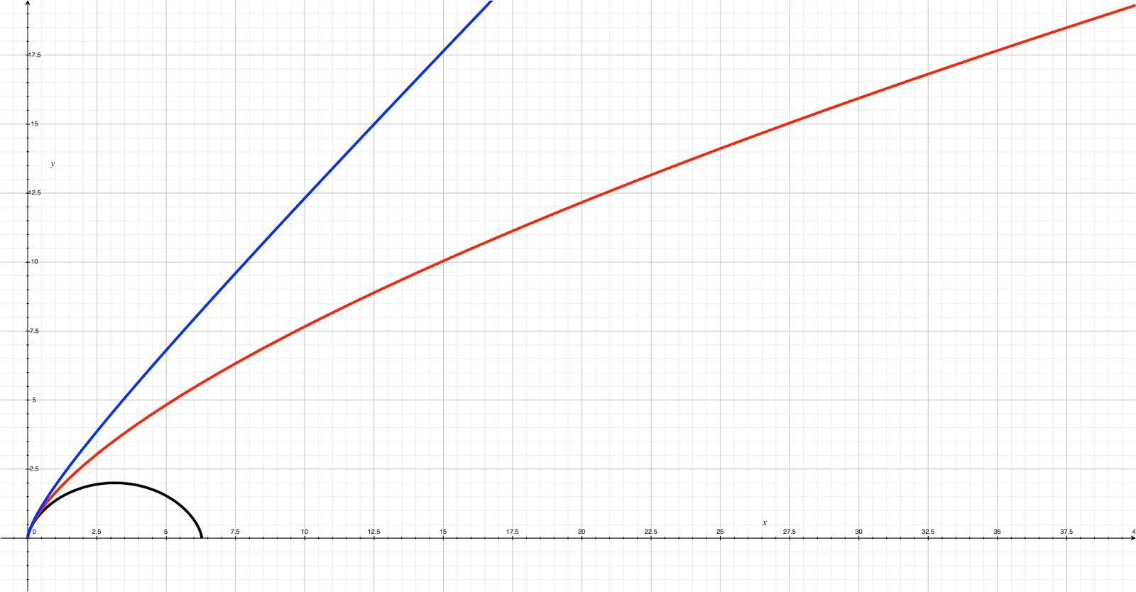
(d) Plot r as a function of t for all three cases (i.e. use y-axis for r and x-axis for t), and show that in the closed case, the particle turns around and collapse; in the open case, the particle keeps expanding with some asymptotically positive velocity; and in the flat case, the particle reaches an infinite radius but with a velocity that approaches zero.
Let's begin.
(a) In the linear theory, it turns out that the fluid equations simplify such that the density contrast δ satisfies the following second-order differential equation
\[\frac{d^2\delta}{dt^2}+\frac{2\dot{a}}{a} \frac{d\delta}{dt}=4\pi G\overline{\rho}\delta\]
where a(t) is the scale factor of the universe. Notice that remarkably in the linear theory this equation does not contain spatial derivatives. Show that this means that the spatial shape of the density fluctuations is frozen in comoving coordinates, only their amplitude changes. Namely this means that we can factorize
\[\delta (x,t)=D(t)\tilde{\delta}(x)\]
where δ ̃(x) is arbitrary and independent of time, and D(t) is a function of time and valid for all x. D(t) is not arbitrary and must satisfy a differential equation. Derive this differential equation.
Let's start with our equation:
\[\frac{d^2\delta}{dt^2}+\frac{2\dot{a}}{a} \frac{d\delta}{dt}=4\pi G\overline{\rho}\delta\]
Now, let's use the second equate to substitute in for delta.
\[\frac{d^2D(t)\tilde{\delta}(x)}{dt^2}+\frac{2\dot{a}}{a} \frac{dD(t)\tilde{\delta}(x)}{dt}=4\pi G\overline{\rho}D(t)\tilde{\delta}(x)\]
Now \(\tilde{\delta}\) cancels.
\[\frac{d^2D(t)}{dt^2}+\frac{2\dot{a}}{a} \frac{dD(t)}{dt}=4\pi G\overline{\rho}D(t)\]
This resultant equation is entirely dependent upon t, as x does not appear anywhere in it, thus it is time independent, and is our differential equation of interest.
(b) Now let us consider a matter dominated flat universe, so that \(\overline{\rho}(t)=a^{-3}\rho_{c,0}\) where \(\rho_{c,0}\) is the critical density today, \(3H_0^2/8\pi G\) as in Worksheet 11.1 (aside: such a universe sometimes is called the Einstein-de Sitter model). Recall that the behaviour of the scale factor of this universe can be written \(a(t)=(3H_0 t/2)^{2/3}\), which you learned in previous worksheets, and solve the differential equation for D(t). Hint: you can use the ansatz \(D(t)\propto t^q\) and plug it into the equation that you derived above; and you will end up with a quadratic equation for q. There are two solutions for q, and the general solution for D is a linear combination of two components: One gives you a growing function in t, denoting it as \(D_+ (t)\); another decreasing function in t, denoting it as \(D_- (t)\).
We will start with the equation from before.
\[\frac{d^2D(t)}{dt^2}+\frac{2\dot{a}}{a} \frac{dD(t)}{dt}=4\pi G\overline{\rho}D(t)\]
We now substitute in for D(t) and \(\overline{\rho}\).
\[\frac{d^2t^q}{dt^2}+\frac{2\dot{a}}{a} \frac{dt^q}{dt}=4\pi G\rho_{c,0}a^{-3}t^q\]
Now, let's focus on the \(\frac{\dot{a}}{a}\) term.
We are told that \(a(t)=(3H_0 t/2)^{2/3}\), so:
\[\frac{\dot{a}}{a}=\frac{2}{3t}\]
Plugging this in, we get:
\[\frac{d^2t^q}{dt^2}+\frac{4}{3t} \frac{dt^q}{dt}=\frac{16\pi G\rho_{c,0}}{9H_0^2 t^2}t^q\]
Taking our derivatives, we get:
\[q(q-1)t^{q-2}+\frac{4qt^{q-2}}{3}=\frac{16\pi G\rho_{c,0}}{9H_0^2}t^{q-2}\]
\(t^{q-2}\) cancels, leaving:
\[q^2+\frac{q}{3}=\frac{16\pi G\rho_{c,0}}{9H_0^2}\]
We now substitute in for \(\rho_{c,0}\).
\[q^2+\frac{q}{3}=\frac{16\pi G3H_0^2}{9\pi 8 G H_0^2}\]
This simplifies to:
\[q^2+\frac{q}{3}=\frac{2}{3}\]
Solving for q we get:
\[q=-1,2/3\]
Finalizing this, we get:
\[\boxed{D_+(t)\propto t^{2/3} \text{ } D_-(t)\propto t^{-1}}\]
(c) Explain why the D+ component is generically the dominant one in structure formation, and show that in the Einstein-de Sitter model, \(D_+ (t)\propto a(t)\).
The D+ component will always be dominant, because as t increases, the D- term will go to 0 since \(\infty^{-1}=0\).
Time for just a little more math:
\[D_+(t)\propto t^{2/3}\]
\[a(t)=(3H_0 t/2)^{2/3}\propto t^{2/3}\]
Thus:
\[D_+(t)\propto t^{2/3} \propto a(t)\]
\[\boxed{D_+(t)\propto a(t)}\]
d) Plot r as a function of t for all three cases (i.e. use y-axis for r and x-axis for t), and show that in the closed case, the particle turns around and collapse; in the open case, the particle keeps expanding with some asymptotically positive velocity; and in the flat case, the particle reaches an infinite radius but with a velocity that approaches zero.
The three cases are an Open Universe (Blue), a Flat Universe (Red), and an a Closed Universe (Black).
I worked with B. Brzycki and N. James on this (last) problem.


